lm2: Simple Linear Regression (Cloze with Theory and Application)

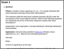
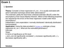
Theory: Consider a linear regression of y on x. It is usually estimated with which estimation technique (three-letter abbreviation)?

This estimator yields the best linear unbiased estimator (BLUE) under the assumptions of the Gauss-Markov theorem. Which of the following properties are required for the errors of the linear regression model under these assumptions?

Application: Using the data provided in linreg.csv estimate a linear regression of y on x. What are the estimated parameters?

Intercept:

Slope:

In terms of significance at 5% level:

Theory: Linear regression models are typically estimated by ordinary least squares (OLS). The Gauss-Markov theorem establishes certain optimality properties: Namely, if the errors have expectation zero, constant variance (homoscedastic), no autocorrelation and the regressors are exogenous and not linearly dependent, the OLS estimator is the best linear unbiased estimator (BLUE).

Application: The estimated coefficients along with their significances are reported in the summary of the fitted regression model, showing that y increases significantly with x (at 5% level).


Call:
lm(formula = y ~ x, data = d)

Residuals:
     Min       1Q   Median       3Q      Max 
-0.50503 -0.17149 -0.01047  0.13726  0.69840 

Coefficients:
             Estimate Std. Error t value Pr(>|t|)
(Intercept) -0.005094   0.023993  -0.212    0.832
x            0.558063   0.044927  12.421   <2e-16

Residual standard error: 0.2399 on 98 degrees of freedom
Multiple R-squared:  0.6116,    Adjusted R-squared:  0.6076 
F-statistic: 154.3 on 1 and 98 DF,  p-value: < 2.2e-16

Code: The analysis can be replicated in R using the following code.

## data
d <- read.csv("linreg.csv")
## regression
m <- lm(y ~ x, data = d)
summary(m)
## visualization
plot(y ~ x, data = d)
abline(m)

Theory: Consider a linear regression of y on x. It is usually estimated with which estimation technique (three-letter abbreviation)?

This estimator yields the best linear unbiased estimator (BLUE) under the assumptions of the Gauss-Markov theorem. Which of the following properties are required for the errors of the linear regression model under these assumptions?

Application: Using the data provided in linreg.csv estimate a linear regression of y on x. What are the estimated parameters?

Intercept:

Slope:

In terms of significance at 5% level:

Theory: Linear regression models are typically estimated by ordinary least squares (OLS). The Gauss-Markov theorem establishes certain optimality properties: Namely, if the errors have expectation zero, constant variance (homoscedastic), no autocorrelation and the regressors are exogenous and not linearly dependent, the OLS estimator is the best linear unbiased estimator (BLUE).

Application: The estimated coefficients along with their significances are reported in the summary of the fitted regression model, showing that y decreases significantly with x (at 5% level).


Call:
lm(formula = y ~ x, data = d)

Residuals:
     Min       1Q   Median       3Q      Max 
-0.48304 -0.14595 -0.00285  0.14840  0.61220 

Coefficients:
            Estimate Std. Error t value Pr(>|t|)
(Intercept)  0.01095    0.02348   0.466    0.642
x           -0.69632    0.04031 -17.272   <2e-16

Residual standard error: 0.233 on 98 degrees of freedom
Multiple R-squared:  0.7527,    Adjusted R-squared:  0.7502 
F-statistic: 298.3 on 1 and 98 DF,  p-value: < 2.2e-16

Code: The analysis can be replicated in R using the following code.

## data
d <- read.csv("linreg.csv")
## regression
m <- lm(y ~ x, data = d)
summary(m)
## visualization
plot(y ~ x, data = d)
abline(m)

Theory: Consider a linear regression of y on x. It is usually estimated with which estimation technique (three-letter abbreviation)?

This estimator yields the best linear unbiased estimator (BLUE) under the assumptions of the Gauss-Markov theorem. Which of the following properties are required for the errors of the linear regression model under these assumptions?

Application: Using the data provided in linreg.csv estimate a linear regression of y on x. What are the estimated parameters?

Intercept:

Slope:

In terms of significance at 5% level:

Theory: Linear regression models are typically estimated by ordinary least squares (OLS). The Gauss-Markov theorem establishes certain optimality properties: Namely, if the errors have expectation zero, constant variance (homoscedastic), no autocorrelation and the regressors are exogenous and not linearly dependent, the OLS estimator is the best linear unbiased estimator (BLUE).

Application: The estimated coefficients along with their significances are reported in the summary of the fitted regression model, showing that x and y are not significantly correlated (at 5% level).


Call:
lm(formula = y ~ x, data = d)

Residuals:
     Min       1Q   Median       3Q      Max 
-0.60164 -0.14469  0.00875  0.13215  0.52337 

Coefficients:
             Estimate Std. Error t value Pr(>|t|)
(Intercept) -0.004520   0.023506  -0.192    0.848
x           -0.001162   0.039513  -0.029    0.977

Residual standard error: 0.2326 on 98 degrees of freedom
Multiple R-squared:  8.82e-06,  Adjusted R-squared:  -0.0102 
F-statistic: 0.0008643 on 1 and 98 DF,  p-value: 0.9766

Code: The analysis can be replicated in R using the following code.

## data
d <- read.csv("linreg.csv")
## regression
m <- lm(y ~ x, data = d)
summary(m)
## visualization
plot(y ~ x, data = d)
abline(m)