R/exams for Blended Learning in a Mathematics 101 Course
Motivation
Many statisticians regularly teach large lecture courses on statistics, probability, or mathematics for students from other fields such as business and economics, social sciences and psychology, etc. A common challenge in such courses is that many variations of similar exercises are needed for written exams, online tests conducted in learning management systems (LMS, such as Moodle, Blackboard, etc.), or live quizzes with voting via smartphones or tablets.
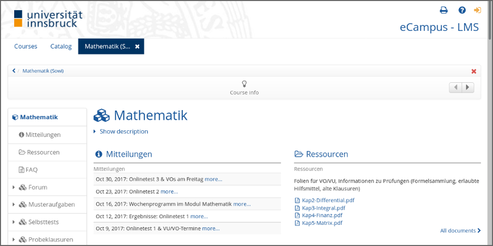
Here, it is shown how the Department of Statistics at Universität Innsbruck manages the first-year mathematics 101 course for economics and business students, attended by about 500 to 1,000 students per semester. The course is accessible through the university’s LMS (an OpenOlat system), including anonymous “Guest access” for most materials. So you can either look at the screen shots presented below in this blog post or try out the course yourself: https://lms.uibk.ac.at/url/RepositoryEntry/4495638563?guest=true. (Notes: The course materials are in German but also non-German-speakers should get a good impression of how things are tied together. The online tests contain mathematical equations in MathML which is displayed by browsers with MathML support like Firefox or Safari - but not Chrome.)
Course overview
As highschool knowledge about mathematics is rather heterogeneous among the students, the course has been designed so that they can learn either synchronously (in a classical lecture that is also streamed live) or asynchronously (with a textbook and/or screencasts). This way students can decide which parts of the content just need reviewing and which need deepening. Similarly, they can get feedback (not directly relevant for their grade) during lecture and tutorial sessions synchronously or asynchronously “in their own time”. Finally, the assessment is also done in two parts: online tests that they can do over the course of the semester (at any time within a 3.5-day window each) and a classical written exam at the end of the semester.
| Learning | Feedback | Assessment | |
|---|---|---|---|
| Synchronous | Lecture Live stream |
Live quiz (+ Tutorial) |
Written exam |
| Asynchronous | Textbook Screencast |
Self test (+ Forum) |
Online test |
Subsequently, it will be discussed how the different feedback and assessment formats are generated with R/exams from the same pool of exercise templates.
Exercises
The core of the course are about 400 dynamic exercise templates where students have to compute some number based on a problem description or a short story. Some examples from this pool have also been translated into English and included in R/exams, e.g., deriv, lagrange, hessian. Almost all of these exercises have been established as num exercises first (with numeric result, employed in online tests) and then converted to single-choice format (schoice, see e.g. deriv2) as this format can be easily scanned automatically in written exams. Additionally, there are about 70 dynamic multiple-choice questions (mchoice) that are used either in online tests or live quizzes.
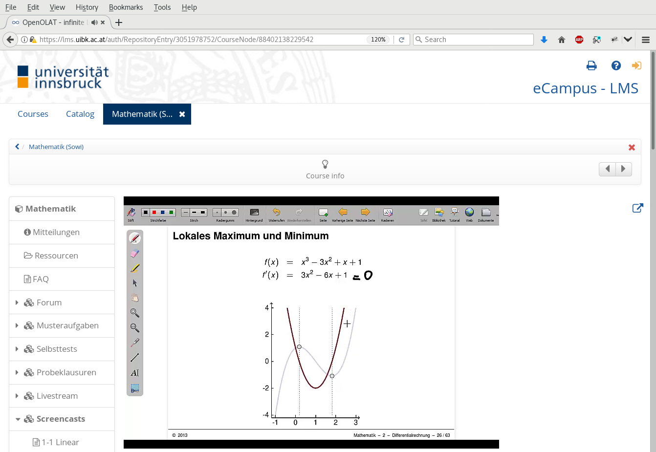
As illustrated in the following, these exercises are the thread running through the enitre course, starting with the lecture slides where typically one static snapshot from an exercise is used (potentially with some additional explanations, incremental slides, graphics, etc.) Below we show screenshots from such a curve sketching exercise in the screencasts (based on the slides). It depicts a simple cubic polynomial of type a x3 + b x2 + c x + d for which the two local optima and the inflection point have to be found.

Online test
The corresponding dynamic exercise templates can then be used in an online test. In fact, here there are three dynamic templates that draw different coefficients a, b, c, and d and either ask for the function value f(x) in one of the local optima (A or C), or the second derivative f’‘(x) in one of the local optima (A or C), or the slope f’(x) in the inflection point B.
In the screenshots below the second derivative f’‘(x) in C is demanded, but the argument x is C incorrectly entered/saved by the student, prompting OpenOlat to display the full correct approach to the solution.


To import an online test into OpenOlat, an XML-based exchange format by the IMS Global Learning Consortium is used: IMS Question & Test Interoperability, Version 1.2 (QTI 1.2). The R/exams function exams2qti12() generates a zipped XML file that can be imported into OpenOlat as a complete online test. To do so we first set up a list of exercises à la:
otest <- list(
  c("deriv-poly.Rnw", "deriv-sqrt.Rnw", "deriv-exp.Rnw", ...),
  c("graph-deriv-A.Rnw", "graph-deriv-B.Rnw", "graph-deriv-C.Rnw"),
  ...
)
And then exams2qti12() can proceed to draw many replications from this combining two forms of randomization: (a) Sampling one item from a given vector of exercise templates (e.g., here the deriv-*.Rnw templates for the first item). (b) In each .Rnw template random numbers are drawn and inserted into the exercise (e.g., the coefficients a, b, c, d in the cubic polynomial). For example:
exams2qti12(otest, n = 500, name = "Mathematik-Onlinetest-01",
  solutionswitch = FALSE, maxattempts = 2, cutvalue = 1000)
draws 500 random versions for each of the items in the test. We don’t show the correct solution approach at the end (only the correct numeric result, solutionswitch = FALSE) but allow our students to attempt each item within the test twice (i.e., one wrong attempt is tolerated). Because individual tests cannot be passed or failed (they just collect points for the overall course), we set cutvalue = 1000 which can never be attained. Due to the large exercise pools and the large number of random variations, the students cannot simply copy a single number or a certain solution formula. Of course, during a 3.5-day test it is possible to help each other and in fact we encourage the students to form small learning groups.
Further control arguments of exams2qti12() include the number of points and the eval strategy (e.g., for negative points upon incorrect results etc.). See ?exams2qti for more technical details and also for an example you can run yourself based on exercises from the template gallery.
In addition to the online tests (= assessment) we employ self tests (= feedback), either in the form of selected demo exercises (“Musteraufgaben”) for which the full solution approach is shown (solutionswitch = TRUE), short tests that sample exercises from almost the entire exercise pool (“Selbsttests”), or “mock exams” based on past written exams (“Probeklausuren”).
| Course element |
Item type |
Templates per item |
Full solution |
Show points during test? |
Time (min.) |
Attempts per item |
Attempts per test |
Purpose |
|---|---|---|---|---|---|---|---|---|
| Online test | num or mchoice |
3-20 | x | 2 | 1 | Assessment during semester |
||
| Demo exercises (Musteraufgaben) |
num or mchoice |
1 | x | x | 1 | ∞ | Feedback after lecture |
|
| Self test (Selbsttest) |
schoice | 3-20 | x | 1 | ∞ | Feedback during semester |
||
| Mock exam (Probeklausur) |
schoice | 1 | 90 | ∞ | ∞ | Feedback before exam |
As the written exams use single-choice versions of the exercises, the latter two test types also practice using this item type (see the screenshot below).

Written exam
The course ends in a “strict” written exam (“Gesamtprüfung”) in the sense that now each student really has to solve his/her own exam without further help in a time window of 90 minutes. The function employed for generating the PDF files is exams2nops() and its usage is illustrated in detail in the tutorial on written exams.
First, a vector (as opposed to a list) of exercises is set up à la:
gp <- c(
  "deriv-sqrt.Rnw",
  "graph-deriv-B.Rnw",
  ...
)
Thus, for written exams we assure that every student gets the same exercise template, only with some random variations of the numbers/graphics/etc. Thus, we try to make the exam as fair as possible while assuring that cheating is very hard. If there are, say, 400 participants in the exam, there are 400 different exams with single-choice exercises. These can be generated (typically after setting a random seed for reproducibility) via:
set.seed(2017-04-05)
exams2nops(gp, n = 400, name = "GP", title = "GP Mathematik",
  institution = "Universit\\\"at Innsbruck", logo = "uibk-logo-bw.png",
  language = "de", course = "403100--200", date = "2017-04-05", reglength = 7,
  pages = c("/path/to/formulary.pdf", "/path/to/normal-table.pdf"))
Thus, in addition to some information about course/exam, we specify the language (German), length of the registration ID (7 digits), and add PDF pages with the formulary and normal tables. The first few pages of one of the resulting PDFs are displayed below. More details on the evaluation process can be found in the exams2nops tutorial.


A very nice benefit of using R/exams here is that we can share an interactive online “mock exam” (“Probeklausur”) in addition to the PDF version in the exam archive. This can again be generated by exams2qti12() with time limit and evaluation settings corresponding to the actual written exam:
exams2qti12(gp, n = 10, name = "Mathematik-GP-2017-04-05",
  maxattempts = Inf, cutvalue = 18, solutionswitch = FALSE,
  points = 2, eval = list(partial = FALSE, negative = -0.25),
  duration = 90)
The screen shots below show first the interactive version of the mock exam and then one of the PDFs in the resources archive.


Live quiz
Finally, the same exercise templates can also be imported into live quizzes when the audience response system ARSnova is used (see https://arsnova.eu/). As we do not use the system for assessment but only for feedback it is not as important to have a lot of random variation in the exercises, but it certainly helps to avoid duplication across courses taught in parallel or in subsequent semesters. Moreover, the R/exams function exams2arsnova() can directly import the drawn exercises into ARSnova using its REST interface (via Rcurl and suitable JSON data). Alternatively, JSON files can be generated on the hard disk and subsequently imported manually.
As an illustration we use again a vector of exercise templates and export random draws from these directly into a previously-generated ARSnova session (using one session for the enitre semester). Authentication can be done through the JSESSIONID.
quiz <- c("deriv-sqrt.Rnw", "graph-deriv-B.Rnw", ...)
exams2arsnova(quiz, name = "Quiz", url = "https://arsnova.uibk.ac.at",
  sessionkey = "79732490", jsessionid = "34A6B8C1D83CB7D0EC66F14DA7044DB1",
  fix_choice = FALSE, abstention = FALSE)
The students can then view the exercises on the mobile phones or tablets, practicing for the exam, followed by a phase of peer instruction to resolve remaining problems.


Exercises like shown in the two screenshots above are used for exam practice during lecture or tutorial sessions. Additionally, knowledge quiz questions are frequently used for checking whether the students can follow the lecture or not. These are typically in the form of multiple-choice questions where each subitem can either be true or false. See gaussmarkov for a worked example.
Summary
This blog post has shown how the same pool of exercises can be used flexibly for different elements of a large-lecture course. Over the last years we experimented quite a bit with these and kept those elements we (or the students) found useful but discontinued using others. Of course, the hard part is establishing the large exercise pool but then R/exams enables us to try out different formats fairly easily.
If you have further questions about these tools or want to let us know how you use R/exams in your course, please get in touch! Either via our forum, StackOverflow, Twitter, or simply by e-mail.